
4.1 Activity - Taxonomy Profiling Spreadsheet
4.1.1 Purpose
Here we will have a hands-on experience with real taxonomy profiling data! We will explore the Kraken2 output for Zymo Gut Microbiome Standard and optionally compare to the Zymo Human Fecal Reference profile. We will introduce concepts of taxa and their relationships, begin familiarizing ourselves with data analysis goals to quantify the proportion of classified and unclassified species, identify the most abundant species, etc.
See accompanying slides.
4.1.2 Learning Objectives
- Explore taxonomy with Kraken 2 taxonomic assignment output.
- Compare and contrast the taxonomy between the Zymo Gut Microbiome Standard and the Zymo Human Fecal Reference.
4.1.3 Introduction
Metagenomics is the direct analysis of the genomes attained through genome sequencing of an environmental sample (soil, water, gut, etc). The purpose of the taxonomic classification of metagenomic sequences is to catalog, classify and identify the species inhabiting a given environment. In the process, we may even identify new species! After sampling, DNA extraction, DNA sequencing, and genome assembly, genome annotation is used to assign taxonomy to the sequenced DNA. Here is where the tool Kraken 2 comes in; Kraken 2 is a taxonomic classification tool which assigns taxonomy to sequencing reads.
4.1.4 Activity 1 – Explore Zymo Gut Standard Metagenomic Diversity
The sample used in this activity is the Zymo Gut Microbiome Standard, sequenced by Pacific Biosciences using PacBio Sequel II Instrument, and corresponds to sequencing read file SRR13128014. A subset of this data is used in this Activity.
Estimated time: 25 min
4.1.4.1 Instructions
- Access tax-data-gut.tsv and open it with Google Sheets here.
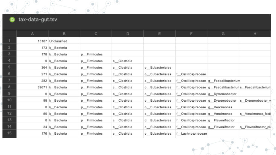
- Identify what information is provided in columns of the tax-data-gut taxonomy file.
- Col A = Counts
- Cols B-H = Taxonomic ranks k(Kingdom), p(Phylum), c(Class), o(Order), f(Family), g(Genus) and s(Species)
- Each row corresponds to a different taxa. There are 153 taxa that were classified for this sample.
- Create a header row and enter the above column information.
4.1.4.2 Questions
1. Evaluate what proportion of data was taxonomically classified.
- Insert a new column A, name it "Calculations", and temporarily use it for calculations. | 1A. How many total counts are there? |
|---|
- In e.g. In cell A2, calculate the sum of all reads observed in the sample.| 1B. What percentage of reads are unclassified? |
|---|
- In e.g. In cell A3, determine the percentage of unclassified reads.| 1C. What percentage of reads are classified? |
|---|
- In e.g. cell A4, determine the percentage of classified reads.2. Identify abundant taxa (those at >1%).
a. Select columns B through I.
b. In the Data menu, select “Sort range by column B (Z to A)”.
c. Insert a new column C, name it “% abundance”, and use it for temporary calculations.
d. In the new column C, calculate % abundance for each row by dividing each count value by the total number of reads and multiplying by 100.
e. Quantify abundant taxa.| 2A. How many abundant taxa (at >1%) do you observe? |
|---|
3. List the abundant taxa you identified in a table below.
- To consolidate the different abundant taxa, in e.g. new column D, copy the lower taxonomic rank identified for the abundant (at >1%) taxa.
- Then, enter the results into a table below.| % abundance | Taxonomy |
|---|---|
| 20.1 | s_Faecalibacterium_prausnitzii |
| 4. How do your results overall compare with the expected taxa and % abundance from the Zymo gut standard? |
|---|
- Compare your results with the expected taxa and abundance for the Zymo gut standard documentation?**
- Note, the Kraken 2 output does not distinguish different E. coli strains, so just combine them all into a single E. coli group!
| 5. Calculate ‘Low abundance’ for < 1% abundant taxa by adding together the taxa at <1%. What percentage of reads are classified as low abundance taxa? |
|---|
| 6. Create a barplot of % abundance for your 12 abundant taxa via Insert Chart. Paste your barplot of % abundance for the 12 most abundant taxa below. |
|---|
4.1.5 Activity 2 (OPTIONAL) – Compare results with the Zymo Fecal Reference
Estimated time: 20 min
4.1.5.1 Instructions
In this activity, repeat the steps of the Activity 1 above, but now using the tax_data_fecal.tsv dataset corresponding to the Zymo fecal reference. The tax_data_fecal.tsv dataset comes from a real human fecal sample, in contrast to the tax_data_gut.tsv sample you explored in the Activity 1, which corresponds to cultured and pooled known species combined at specific proportions to make up a predictable standard population.
- Perform the excercises from Activity 1 using the tax_data_fecal data, then, use questions below to compare the two datasets.
- See D6323 Zymo Fecal Microbiome References documentation (pg. 4) in the Resources section below.
4.1.6 Grading Criteria
- Download this assignment as Microsoft Word (.docx) and upload on Canvas.
- Download your Google Sheet as Microsoft Excel (.xlsx) and upload on Canvas.
4.1.7 Footnotes
Resources
- Google Doc
- D6331 Zymo Gut Microbiome Standard documentation
- D6323 Zymo Fecal Microbiome References documentation
Contributions and Affiliations
- Valeriya Gaysinskaya, Johns Hopkins University
- Gauri Paul, Clovis Community College
- Frederick Tan, Johns Hopkins University
Last Revised: July 2025